Applying a circular moving window filter to raster data in R

The raster package for R provides a variety of functions for the analysis of raster GIS data. The focal() function is very useful for applying moving window filters to such data. I wanted to calculate a moving window mean for cells within a specified radius, but focal() did not provide a built-in option for this. The following code generates an appropriate weights matrix for implementing such a filter, by using the matrix as the w argument of focal().

require(raster)
#function to make a circular weights matrix of given radius and resolution
#NB radius must me an even multiple of res!
make_circ_filter<-function(radius, res){
  circ_filter<-matrix(NA, nrow=1+(2*radius/res), ncol=1+(2*radius/res))
  dimnames(circ_filter)[[1]]<-seq(-radius, radius, by=res)
  dimnames(circ_filter)[[2]]<-seq(-radius, radius, by=res)
  sweeper<-function(mat){
    for(row in 1:nrow(mat)){
      for(col in 1:ncol(mat)){
        dist<-sqrt((as.numeric(dimnames(mat)[[1]])[row])^2 +
          (as.numeric(dimnames(mat)[[1]])[col])^2)
        if(dist<=radius) {mat[row, col]<-1}
      }
    }
    return(mat)
  }
out<-sweeper(circ_filter)
return(out)
}

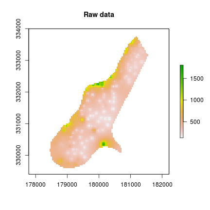
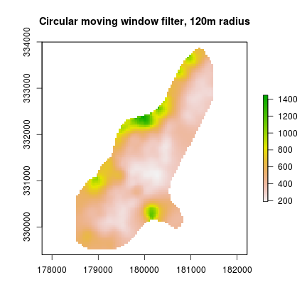
This example uses a weighs matrix generated by make_circ_filter() to compute a circular moving average on the Meuse river grid data. For a small raster like this, the function is more than adequate. For large raster datasets, it’s quite slow though.

#make a  circular filter with 120m radius, and 40m resolution
cf<-make_circ_filter(120, 40)

#test it on the meuse grid data
f <- system.file("external/test.grd", package="raster")
r <- raster(f)

r_filt<-focal(r, w=cf, fun=mean, na.rm=T)

plot(r, main="Raw data") #original data
plot(r_filt, main="Circular moving window filter, 120m radius") #filtered data

Using R for spatial sampling, with selection probabilities defined in a raster

The raster package for R provides a range of GIS-like functions for analysing spatial grid data. Together with package sp, and several other spatial analysis packages, R provide a quite comprehensive set of tools for manipulating and analysing spatial data.

I needed to randomly select some locations for field sampling, with inclusion probabilities based on values contained in a raster. The code below did the job very easily.

library(raster)

#an example raster from the raster package
f <- system.file("external/test.grd", package="raster")
r<-raster(f)

plot(r)

#make a raster defining the desired inclusion probabilities 
#for the all locations available for sampling
probrast<-raster(r)
#inclusion probability for cells with value >=400 
#will be 10 times that for cells with value <400
probrast[r>=400]<-10 
probrast[r<400]<-1
#normalise the probability raster by dividing 
#by the sum of all inclusion weights:
probrast<-probrast/sum(getValues(probrast), na.rm=T)

#confirm sum of probabilities is one
sum(getValues(probrast), na.rm=T)

#plot the raster of inclusion probabilities
plot(probrast, col=c(gray(0.7), gray(0.3)))

#a function to select N points on a raster, with 
#inclusion probabilities defined by the raster values.
probsel<-function(probrast, N){
  x<-getValues(probrast)
  #set NA cells in raster to zero
  x[is.na(x)]<-0
  samp<-sample(nrow(probrast)*ncol(probrast), size=N, prob=x)
  samprast<-raster(probrast)
  samprast[samp]<-1 #set value of sampled squares to 1
  #convert to SpatialPoints
  points<-rasterToPoints(samprast, fun=function(x){x>0})
  points<-SpatialPoints(points)
 return(points)
}

#select 300 sites using the inclusion probabilities 
#defined in probrast
samppoints<-probsel(probrast, 300)
plot(probrast, col=c(gray(0.7), gray(0.3)), axes=F)
plot(samppoints, add=T, pch=16, cex=0.8, col="red")

Here’s the result. Note the higher density of sampled points (red) within the parts of the raster with higher inclusion probability (dark grey).