A simple method for including Māori vowels in R plots

My Kiwi buddy Andrew Gormley was having trouble including the Māori language vowels with macrons (ā, ē, ī, ō, ū) in his R plots.

Macrons in R labels for Māori words – I use unicodes. ā = u0101, ē = u0113, ī = u012B, ō = u014D, ū = u016B.
So for a margin text for Tūī, dont use mtext("Tui",3), just sub in the unicodes, e.g. mtext("Tu016Bu012b", 3).
Maybe there is a better/easier way?

— Andrew Gormley (@EcolModAG) November 22, 2017

I wrote a quick R function “maorify.r” (code in the gist below), which provides a simple method for including these characters in R plots without having to type out the unicode in full each time. I’m sure there’s a simpler or more general purpose way to do this, but it does work. Perhaps it might be useful to anyone analysing Kiwi data with R.

	#function to substitute vowels with Maori macrons into text strings in R
	#there's probably a fancier way to do this, but it works OK.
	#just precede vowels requiring a macron with '@' and the function will substitute the appropriate vowel with macron.
	#Handy for graph labelling etc.
	maorify<-function(x){
	x<-gsub("@a","\u0101", x) #macron a
	x<-gsub("@e","\u0113", x) #macron e
	x<-gsub("@i","\u012B", x) #macron i
	x<-gsub("@o","\u014D", x) #macron o
	x<-gsub("@u","\u016B", x) #macron u
	return(x)
	}
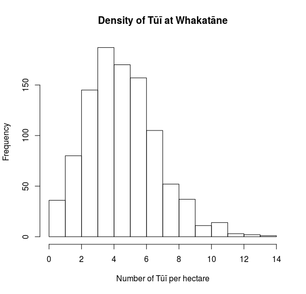
	#Example usage
	hist(rpois(1000, 5), xlab=maorify("Number of T@u@i per hectare"),
	main=maorify("Density of T@u@i at Whakat@ane"))

view raw maorify.R hosted with ❤ by GitHub

 

 

 

Adding phylopic.org silhouettes to R plots

Over at phylopic.org there is a large and growing collection of silhouette images of all manner of organisms – everything from Emus to Staphylococcus. The images are free (both in cost, and to use), are available in vector (svg) and raster (png) formats at a range of resolutions, and can be searched by common name, scientific name and (perhaps most powerfully) phylogenetically.

[EDIT: as two commenters have pointed out, not all phylopic images are totally free of all restrictions on use or reuse: some require attribution, or are only free for non-commercial use. It’s best to check before using an image, either directly at the phylopic webpage, or by using the phylopic API]

Phylopic images are useful wherever it is necessary to illustrate exactly which taxon a graphical element pertains to, as pictures always speak louder than words.

Below I provide an example of using phylopic images in R graphics. I include some simple code to automatically resize and position a phylopic png within an R plot. The code is designed to preserve the original png’s aspect ratio, and to place the image at a given location within the plot.

	library(png)
	library(RCurl)
	#I got these free png silhouettes of red fox and rabbit from phylopic.org
	foxurl<-"http://phylopic.org/assets/images/submissions/51b1b6e4-129d-41a6-bbbd-c3fab459c25f.1024.png&quot;
	raburl<-"http://phylopic.org/assets/images/submissions/1e15411c-5394-4a9d-a209-76c8ac0c331d.1024.png&quot;
	fox_logo <- readPNG(getURLContent(foxurl))
	rab_logo <- readPNG(getURLContent(raburl))
	#utility function for embedding png images at specified fractional sizes in R plots
	#places the logo centred on a specified fraction of the the usr space,
	#and sizes appropriately (respects aspect ratio)
	logoing_func<-function(logo, x, y, size){
	dims<-dim(logo)[1:2] #number of x-y pixels for the logo (aspect ratio)
	AR<-dims[1]/dims[2]
	par(usr=c(0, 1, 0, 1))
	rasterImage(logo, x-(size/2), y-(AR*size/2), x+(size/2), y+(AR*size/2), interpolate=TRUE)
	}
	#Demo: a time-series plot of fake fox and rabbit abundance data with phylopic logos overlaid
	pdf("fox_plot.pdf", width=6, height=10)
	layout(matrix(1:2, nrow=2))
	set.seed(122)
	plot(y=50*cumprod(exp(rnorm(30, 0.05, 0.1))), x=1981:2010, xlab="Time", pch=16,
	ylab="Fox abundance", las=1, col="tomato", lwd=2, type="o", ylim=c(0, 150))
	#adding a fox silhouette logo near the bottom righthand corner
	logoing_func(fox_logo, x=0.10, y=0.90, size=0.15)
	title(main="Index of fox abundance, 1981-2010")
	plot(y=50*cumprod(exp(rnorm(30, -0.05, 0.2))), x=1981:2010, xlab="Time", pch=17,
	ylab="Rabbit abundance", las=1, col="orange", lwd=2, type="o", ylim=c(0, 150))
	#adding a fox silhouette logo near the bottom righthand corner
	logoing_func(rab_logo, x=0.10, y=0.90, size=0.15)
	title(main="Index of rabbit abundance, 1981-2010")
	dev.off()

view raw logo_add.r hosted with ❤ by GitHub

I should also point readers to Scott Chamberlain‘s R package fylopic, which provides the ability to make use of the phylopic API from within R, including the ability to search for and download silhouettes programatically.

If you find phylopic useful, I’m sure they would appreciate you providing them with silhouettes of your study species. More information on how to submit your images can be found here.

Applying a circular moving window filter to raster data in R

The raster package for R provides a variety of functions for the analysis of raster GIS data. The focal() function is very useful for applying moving window filters to such data. I wanted to calculate a moving window mean for cells within a specified radius, but focal() did not provide a built-in option for this. The following code generates an appropriate weights matrix for implementing such a filter, by using the matrix as the w argument of focal().

require(raster)
#function to make a circular weights matrix of given radius and resolution
#NB radius must me an even multiple of res!
make_circ_filter<-function(radius, res){
  circ_filter<-matrix(NA, nrow=1+(2*radius/res), ncol=1+(2*radius/res))
  dimnames(circ_filter)[[1]]<-seq(-radius, radius, by=res)
  dimnames(circ_filter)[[2]]<-seq(-radius, radius, by=res)
  sweeper<-function(mat){
    for(row in 1:nrow(mat)){
      for(col in 1:ncol(mat)){
        dist<-sqrt((as.numeric(dimnames(mat)[[1]])[row])^2 +
          (as.numeric(dimnames(mat)[[1]])[col])^2)
        if(dist<=radius) {mat[row, col]<-1}
      }
    }
    return(mat)
  }
out<-sweeper(circ_filter)
return(out)
}

This example uses a weighs matrix generated by make_circ_filter() to compute a circular moving average on the Meuse river grid data. For a small raster like this, the function is more than adequate. For large raster datasets, it’s quite slow though.

#make a  circular filter with 120m radius, and 40m resolution
cf<-make_circ_filter(120, 40)

#test it on the meuse grid data
f <- system.file("external/test.grd", package="raster")
r <- raster(f)

r_filt<-focal(r, w=cf, fun=mean, na.rm=T)

plot(r, main="Raw data") #original data
plot(r_filt, main="Circular moving window filter, 120m radius") #filtered data

Mapping georss data using R and ggmap

Readers might recall my earlier efforts at using R and python for geolocation and mapping of realtime fire and emergency incident data provided as rss feeds by the Victorian Country Fire Authority (CFA). My realisation that the CFA’s rss feeds are actually implemented using georss (i.e. they already contain locational data in the form of latitudes and longitudes for each incident), makes my crude implementation of a geolocation process in my earlier python program redundant, if not an interesting learning experience.

I provide here an quick R program for mapping current CFA fire and emergency incidents from the CFA’s georss, using the excellent ggmap package to render the underlying map, with map data from google maps.

Here’s the code:

library(ggmap)
library(XML)
library(reshape)

#download and parse the georss data to obtain the incident locations:
cfaincidents<-xmlInternalTreeParse("http://osom.cfa.vic.gov.au/public/osom/IN_COMING.rss")
cfapoints <- sapply(getNodeSet(cfaincidents, "//georss:point"), xmlValue)
cfacoords<-colsplit(cfapoints, " ", names=c("Latitude", "Longitude"))

#map the incidents onto a google map using ggmap
library(ggmap)
library(XML)
library(reshape)

#download and parse the georss data to obtain the incident locations:
cfaincidents<-xmlInternalTreeParse("http://osom.cfa.vic.gov.au/public/osom/IN_COMING.rss")
cfapoints <- sapply(getNodeSet(cfaincidents, "//georss:point"), xmlValue)
cfacoords<-colsplit(cfapoints, " ", names=c("Latitude", "Longitude"))

#map the incidents onto a google map using ggmap
png("map.png", width=700, height=700)
timestring<-format(Sys.time(), "%d %B %Y, %H:%m" )
titlestring<-paste("Current CFA incidents at", timestring)
map<-get_map(location = "Victoria, Australia", zoom=7, source="google", maptype="terrain")
ggmap(map, extent="device")+ 
  geom_point(data = cfacoords, aes(x = Longitude, y = Latitude), size = 4, pch=17, color="red")+
  opts(title=titlestring)
dev.off()

And here’s the resulting map, showing the locations of tonight’s incidents. Note that this is a snapshot of incidents at the time of writing, and should not be assumed to represent the locations of incidents at other times, or used for anything other than your own amusement or edification. The authoritative source of incident data is always the CFAs own website and rss feeds.