State-space occupancy model using PyMC

I’ve continued my experimentation with PyMC, using it to fit occupancy models to wildlife survey data with imperfect detectability. Chris Fonnesbeck has provided code for a simple, single-survey occupancy model here, which provides a good starting point for experimentation. I wanted to construct my model using the alternative, state-space parameterisation for occupancy models described by Royle and Kéry(2007). Unlike the multi-season, dynamic occupancy model described by Royle and Kéry, I am only fitting a single-season occupancy model, where the site-states (occupied or unoccupied) are assumed to be constant. The model uses a hierarchical approach, where sites are occupied with probability , and the true occupancy states of the sites, are inferred from repeated surveys at each site based on a probabilistic detection model (in this case a simple Bernoulli model, with conditional probability of detection at each survey ). Fitting this model using MCMC has the advantage that a finite-sample estimate of occupancy rates among the sampled sites can be easily computed by sampling from .

from pymc import *
from numpy import *

"""
Alternative implementation of single season occupancy estimation for the Salamander data (from MacKenzie et al. 2006), using a 
state-space approach.

Modified from original example code and data provided by Chris Fonnesbeck at https://github.com/pymc-devs/pymc/wiki/Salamanders
"""


# Occupancy data - rows are sites, with replicate surveys conducted at each site
salamanders = array([[0,0,0,1,1], [0,1,0,0,0], [0,1,0,0,0], [1,1,1,1,0], [0,0,1,0,0], 
                     [0,0,1,0,0], [0,0,1,0,0], [0,0,1,0,0], [0,0,1,0,0], [1,0,0,0,0], 
                     [0,0,1,1,1], [0,0,1,1,1], [1,0,0,1,1], [1,0,1,1,0], [0,0,0,0,0], 
                     [0,0,0,0,0], [0,0,0,0,0], [0,0,0,0,0], [0,0,0,0,0], [0,0,0,0,0], 
                     [0,0,0,0,0], [0,0,0,0,0], [0,0,0,0,0], [0,0,0,0,0], [0,0,0,0,0], 
                     [0,0,0,0,0], [0,0,0,0,0], [0,0,0,0,0], [0,0,0,0,0], [0,0,0,0,0], 
                     [0,0,0,0,0], [0,0,0,0,0], [0,0,0,0,0], [0,0,0,0,0], [0,0,0,0,0], 
                     [0,0,0,1,0], [0,0,0,1,0], [0,0,0,0,1], [0,0,0,0,1]])

# Number of replicate surveys at each site
k = 5

#number of detections at each site (row sums of the data)
y=salamanders.sum(axis=1)

#vector of known/unknown occupancies to provide sensible starting values for latent states, z.
#Equal to 1 if at least 1 detection, otherwise zero.
z_start = y>0

# Prior on probability of detection
p = Beta('p', alpha=1, beta=1, value=0.99)

# Prior on probability of occupancy
psi = Beta('psi', alpha=1, beta=1, value=0.01)

#latent states for occupancy
z = Bernoulli('z', p=psi, value=z_start, plot=False)

#Number of truly occupied sites in the sample (finite-sample occupancy)
@deterministic(plot=True)
def Num_occ(z=z):
   out = sum(z)
   return out

#unconditional probabilities of detection at each site (zero for unoccupied sites, p for occupied sites)
@deterministic(plot=False)
def pdet(z=z, p=p):
    out = z*p
    return out

#likelihood
Y = Binomial('Y', n=k, p=pdet, value=y, observed=True)

Fitting of the model was accomplished by running the following code, which constructs the model, collects some MCMC samples for parameters of interest, and generates plots of the results:

from pylab import *
from pymc import *

import model

#get all the variables from the model file
M = MCMC(model)

#draw samples
M.sample(iter =40000, burn = 20000, thin = 5)

#plot results
Matplot.plot(M)

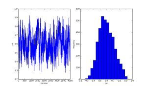
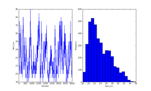
Her are some summary plots (traces and histograms) for the MCMC samples of the parameters and

The same model can easily be fitted using OpenBUGS, with comparable results..

model{
psi~dbeta(1, 1)
p~dbeta(1, 1)
for(i in 1:sites){
   z[i]~dbern(psi)
   pdet[i]<-p*z[i]
  for(j in 1:surveys){
 Y[i,j]~dbern(pdet[i])
   }
  }
}

data
list(
surveys=5,
sites=39,
Y=structure(.Data = 
c(0,0,0,1,1, 
0,1,0,0,0, 
0,1,0,0,0, 
1,1,1,1,0, 
0,0,1,0,0, 
0,0,1,0,0, 
0,0,1,0,0, 
0,0,1,0,0, 
0,0,1,0,0, 
1,0,0,0,0, 
0,0,1,1,1, 
0,0,1,1,1, 
1,0,0,1,1, 
1,0,1,1,0, 
0,0,0,0,0, 
0,0,0,0,0, 
0,0,0,0,0, 
0,0,0,0,0, 
0,0,0,0,0, 
0,0,0,0,0, 
0,0,0,0,0, 
0,0,0,0,0, 
0,0,0,0,0, 
0,0,0,0,0, 
0,0,0,0,0, 
0,0,0,0,0, 
0,0,0,0,0, 
0,0,0,0,0, 
0,0,0,0,0, 
0,0,0,0,0, 
0,0,0,0,0, 
0,0,0,0,0, 
0,0,0,0,0, 
0,0,0,0,0, 
0,0,0,0,0, 
0,0,0,1,0, 
0,0,0,1,0, 
0,0,0,0,1, 
0,0,0,0,1),
 .Dim=c(39,5))
)

PyMC for Bayesian models

BUGS and JAGS have been the main tools I have used for fitting Bayesian statistical models for a long time now. Both have their strengths and weaknesses, but they are extremely useful tools, and I would anticipate that they will continue to develop their capabilities, and remain important components of my statistical toolbox for some time to come.

Recently, I’ve become aware of an alternative platform for Bayesian modelling, that has similar potential to BUGS and it’s dialects – PyMC. PyMC provides a framework for describing and fitting Bayesian statistical models using the Python programming language. Having read the paper describing the software, and consulted the user guide, I decided to have a try at building a simple linear regression model as a test, despite having very limited experience with python. I found that consulting the examples on the PyMC website, as well as the material presented in Abraham Flaxman’s blog very helpful for getting started, and for solving problems along the way.

I started by simulating some data from a very simple Gaussian linear model using R. I’m sure this could be easily done in Python, but for now R will be quicker and easier for me to code:

N<-50
x<-round(runif(N, -20, 20))
y<-rnorm(N, 2*x+ 3, 10)
plot(y~x)
cat(x, sep=", ", fill=T)
cat(y, sep=", ", fill=T)

Running this code resulted in two nicely concatenated vectors of random x and y values generated from the (known) regression model . These random values were easily transferred to the PyMC code for the Bayesian model using cut-and-paste – clumsy, but it works for me…..

Here is the python code for the ordinary linear model, with the randomly generated data (called YY and XX) pasted in. Vague normal priors were assumed for the slope and intercept parameters ( and ), while the standard deviation of the random errors () was assigned a Uniform prior:

## Regression
from pymc import *
from numpy import *

#data
YY = array([-19.23776, 1.559197, 27.90364, -14.94222, -41.34614, 5.857922,  -26.24492, -1.670176, -8.349098, -24.91511, 63.86167, 20.87778, 4.176622, -35.65956, 4.482383, 36.20763, 33.60314, 23.25372, -15.52639, -25.59295, 42.48803, -29.46465, 30.25402, -5.66534, -20.92914, 44.87109, 19.07603, 22.19699, 18.89613, 2.835296, 12.68109, -17.19655, 26.60962, -28.74333, -24.69688,  -19.02279, -31.39471, -17.83819, 15.389, 40.41935, 0.972758, -36.49488,  -2.041068, 23.22597, 1.226252, 11.87125, 36.32597, 29.20536, 16.24043, -0.8978296])

XX = array([-14, -6, 19, -12, -16, 1, -15, -13, 0, -6, 15, 8, 1, -16, -5, 19, 8, 7, -11, -13, 13, -18, 10, -1, -13, 13, 13, 17, 13, 11, 4, -6, 14, -14, 3, -3, -18, -11, 6, 13, -10, -12, -2, 9, -7, -1, 14, 15, 6, -2])

#priors
sigma = Uniform('sigma', 0.0, 200.0, value=20)
alpha = Normal('alpha', 0.0, 0.001, value=0)
beta = Normal('beta', 0.0, 0.001, value=0)

#model
@deterministic(plot=False)
def modelled_yy(XX=XX, beta=beta, alpha=alpha):
    return beta*XX + alpha

#likelihood
y = Normal('y', mu=modelled_yy, tau=1.0/sigma**2, value=YY, observed=True)

The python code for the model saved to a file named regress.py. Generating an MCMC sample from the parameters of model was then just a matter of running the following code within a python shell:

from pylab import *
from pymc import *
import regress
M = MCMC(regress)
M.sample(10000, burn=5000)
Matplot.plot(M)

The code also generates some summary plots (traces and histograms) for each of the parameters. So far so good – it looks like the inferred values for the parameters fairly closely match those that the random data were generated from:

I’ll move onto some more complex models soon, but so far PyMC looks quite promising as a tool for Bayesian modelling. Perhaps a useful strategy for learning will be to construct a variety models of increasing complexity, with a focus on the types of models I use for my research.